
What is LU decomposition?
What happens inside when when your ML model solves a linear system

Every time you call np.linalg.solve(A, b), something elegant happens under the hood. NumPy doesn’t invert the matrix A. Matrix inversion is expensive, numerically fragile for large systems, and wasteful if you need to solve the same system repeatedly.
Instead, it factors A into two simpler matrices and solves in two cheaper steps. That factorization is called LU decomposition.
How does it work?
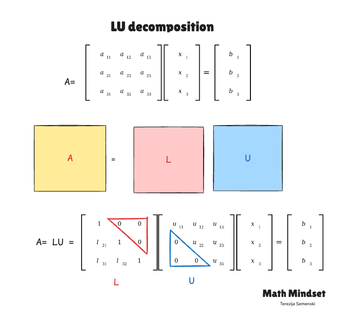
LU decomposition factors a square matrix A into the product of two triangular matrices:
A = L × U
where this factorization exists when all leading principal submatrices of A are nonsingular. In practice, partial pivoting is used to extend this to a broader class of matrices, giving the factorization PA = L × U, where P is a permutation matrix that records row interchanges.
L is lower-triangular: every entry above the diagonal is 0.
U is upper-triangular: every entry below the diagonal is 0.
To solve Ax = b, rewrite it as LUx = b, then solve in two passes:
Step 1: Solve Ly = b using forward substitution (top to bottom, O(n²))
Step 2: Solve Ux = y using back substitution (bottom to top, O(n²))
The one-time factorization costs O(n³). After that, every additional solve costs only O(n²). That is the key advantage over recomputing inverses or refactorizing from scratch.
Example
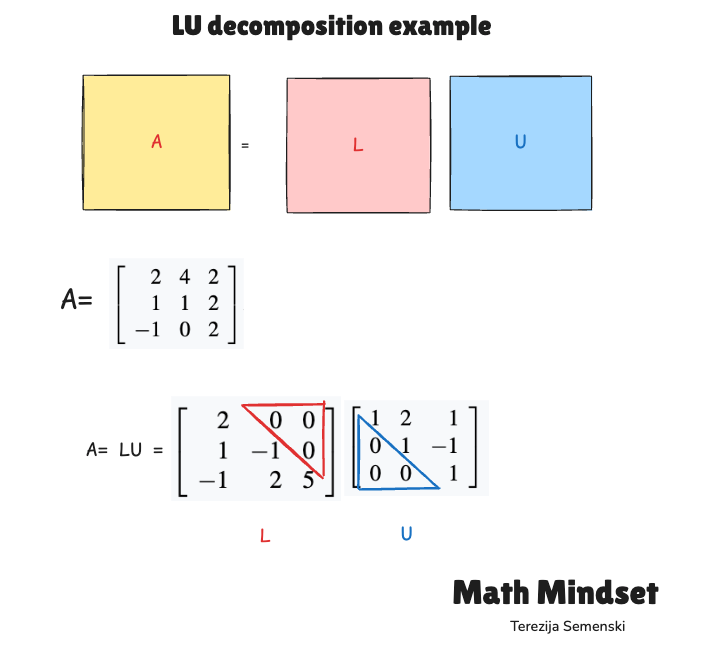
Suppose you have a 3×3 system Ax = b. Without LU decomposition, one alternative is to compute A⁻¹ explicitly and then form the solution as x = A⁻¹b.
This requires O(n³) work just to produce the inverse, followed by an additional O(n²) matrix-vector multiplication, and it tends to accumulate floating-point errors more aggressively than factorization-based methods. For repeated solves, it is both slower and less numerically reliable.
LU decomposition sidesteps this entirely.
You perform Gaussian elimination once to produce L and U. From that point forward, solving for any new right-hand side b is just two triangular solves, each of which runs in O(n²) time.
The real advantage comes from the triangular structure.
A lower-triangular system like Ly = b can be solved by starting at the first equation, which contains only one unknown, and working downward. Each equation introduces exactly one new variable, so you never need to do anything more complex than a single division and a sum.
The same logic applies to Ux = y, just in reverse order.
This is forward and back substitution. It is simple, stable, and fast.
Here is the part that makes it elegant
You factor A once. Then you can solve for any number of right-hand side vectors b₁, b₂, b₃ without ever touching L and U again. Each additional solve costs only O(n²).
If your model trains on 10,000 batches and solves the same linear system at each step, LU decomposition saves you from 10,000 full matrix inversions. The heavy O(n³) cost is paid once. Everything after that is cheap.
This idea, paying a large fixed cost upfront to make repeated operations fast, appears constantly in numerical computing. LU decomposition is one of its clearest and most useful instances.
Why does this matter in ML?
Linear systems appear in more places than most practitioners realize:
Linear regression and least-squares solvers ultimately reduce to solving Ax = b.
Gaussian mixture models fit data by assuming it comes from a blend of several Gaussian distributions. During training, the algorithm needs to measure the shape and spread of each cluster, which requires working with covariance matrices. For each cluster, it needs to compute quantities involving the inverse and determinant of that covariance matrix. LU decomposition handles this efficiently without ever forming the inverse explicitly, which matters a lot when you have many features.
Kalman filters, used in robotics and time-series forecasting, rely on efficient matrix solves at every update step.
Any iterative solver that repeatedly solves Ax = b for different right-hand side vectors amortizes the O(n³) factorization cost across all of them.
The pattern is always the same: factor once, solve many times cheaply.
A note on numerical stability
In practice, LU decomposition is almost always implemented with partial pivoting, which means rows of A are reordered during factorization to keep the arithmetic stable. Without pivoting, small diagonal entries can cause division by near-zero values and introduce large numerical errors. With pivoting, LU decomposition becomes one of the most reliable general-purpose solvers available.
This is why the full factorization is written as PA = LU, where P is a permutation matrix that records the row swaps. NumPy handles this automatically, so in practice you never need to think about it. But understanding why it exists helps you appreciate that numerical linear algebra is not just about mathematical correctness. It is about keeping floating-point arithmetic well-behaved at scale.
Why numerical Linear algebra is its own discipline
The same mathematical problem, solving Ax = b, can be approached many different ways: direct inversion, Gaussian elimination, LU decomposition, Cholesky factorization when A is symmetric positive definite, or iterative methods like conjugate gradient. Each carries different tradeoffs in cost, stability, and memory usage.
LU decomposition sits near the center of this landscape. It is general enough to handle arbitrary square matrices, stable enough for practical use with partial pivoting, and efficient enough that it underlies the default behavior of NumPy, MATLAB, and most scientific computing libraries.
The next time np.linalg.solve() returns an answer in milliseconds, you now know exactly what is happening inside.
P.S. Thank you for reading this far.
That alone puts you in rare company: most people scroll past anything that asks them to think slowly.
The fact that you’re here suggests you already value the kind of thinking this newsletter is about. Share it with someone who values it too. Those people are worth finding.
Comment below and share the newsletter/ issue if you think it is relevant!
Feel free to also follow me on LinkedIn (very active), Instagram(not so active) or X (not so active).
Until next week’s issue, keep learning, keep building, and keep thinking like a mathematician.
-Terezija
Thank you for this deep dive!